
From the Shop: Digital Scales - "The YADRO-Files" : Part 5
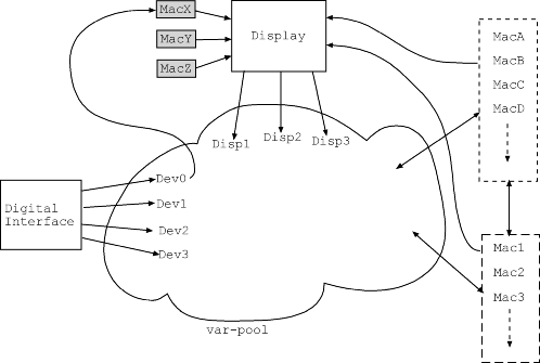
The inner workings of YADRO. A short introduction.Even if you don't want to change YADRO's ego, you should read the first part. As I said, YADRO comes with it's own programming language. That language is a C-like language, that I will call YPL (for YADRO-Programming-Language or Yet Another Digital Read Out Programming Language). The code that drives your display consists of quite a few code snippets or macros that interact. There is a big variable pool every piece of code can access. There are some special function calls that interact with the display. The display itself is quite stupid and knows nothing about scaling, offset etc. Here is a sketch:
The
cloud named var-pool is the storage that keeps all the variables. Every
part of the program or the macros can access and modify them. YADRO does the following:
|
; YADRO-Configuration file ; ; Lines are format sensitive. That means that you should not put blanks ; where you want. They won't be skipped. ; Comments start with a ";" at the leftmost position. This is an example ; for format sensitivity. |
The whole YADRO.CFG consists of a list of instructions. To make your life a bit easier you can have comments between macros or interpreter-commands (you'll see that in a moment). Comments start with a ";" at the leftmost position. But you don't need comments, don't you?
Interp:
  display("ConnectAs", 0, 0);
  display("ConnectAs", 2, 1);
:EndI
|
Everything between the symbols Interp: and :EndI
(on the leftmost!) is directly sent to the interpreter. It is not
stored and can not later be referenced. It is handy for setting things
up.
We need to know what devices are connected and to read from. We tell this the YADRO-engine with display("ConnectAs", 0, 0). Everything influencing the display (or the YADRO-engine) has the command display.
You can connect a physical device at some port to a different logical
device. A physical device is the digital scale, a logical device is
represented by it's value in the variable-pool. To connect the physical
device #0 to the variable#2 write display("ConnectAs", 0, 2).
This way you can break the dependencies between the cables and the
logic behind axis. You can even logically swap axis during runtime. If
your X-axe is connected to dev#0 and your Y-axe to dev#1 you have a display("ConnectAs", 0, 0) and a display("ConnectAs", 1, 1).
If you want (whenever) to flip X and Y, you execute the commands display("ConnectAs", 0, 1) and display("ConnectAs", 1, 0).
You can even logically disconnect devices (if you no longer need to read from it during execution) with a display("DisConnect", 1) (here for dev#1).
Interp:
  display("AxName", 1, "X");
  display("AxName", 2, "Y");
  display("AxName", 3, "Z");

  display("AxSecName", 1, "X (abs)");
  display("AxSecName", 2, "Y (abs)");
  display("AxSecName", 3, "Z (abs)");
:EndI
|
Now
axis need names. They are not hard coded into the program. They are
defined. Internally, axis are numbered from 1…3 (3 axis for now). Axe
number 1 being the topmost. You give names to axis with display("AxName", 1, "X")
(naming axe #1 "X"). Theoretically you can give names you want, but
currently, only a few characters are supported (will add more, have to
design them). The names allowed for now are "X", "Y", "Z" and the
diameter-sign. To get the diam.character, you write "/O".
Because
of YADRO being better, you not only have 3 axes, but 3 primary axis and
3 secondary axis. The later you define with display("AxSecName", 1,
"X"). They are displayed directly below the primary axis, and are very
handy to reflect the absolute value. If you don't define them (same for
primary axis), they will not show.
If you want to remove an axe during runtime, you make a display with an
empty string (eg ""). Don't forget, that YADRO still will read from the
physical device you defined in display("ConnectAs"…).
Interp: fvar Dev0ScalingMetric, Dev0ScalingInch; fvar Dev1ScalingMetric, Dev1ScalingInch; fvar Dev2ScalingMetric, Dev2ScalingInch; fvar PrecisionMetric, PrecisionInch; Dev0ScalingMetric = 1 / 100; Dev0ScalingInch = 1 / (100 * 25.4); Dev1ScalingMetric = 1 / (-20480 / 25.4); Dev1ScalingInch = 1 / -20480; Dev2ScalingMetric = Dev1ScalingMetric; Dev2ScalingInch = Dev1ScalingInch; PrecisionMetric = 2; PrecisionInch = 4; :EndI |
As
I said, there is a variable pool. The variables need to be declared and
defined. Variables do have no scope, they are always global. You might
call this ugly or bad style, but in this case it is OK, because all the
code tends to be monolithic and small.
Variables are defined with fvar
(for float-variable). Currently, there are only floats (long double for
the programmers). The reason why it is wise to define the variables
directly (by Interp:) is, that it is better to define and
declare them at a place the program does not execute again and again.
Albeit the instruction is lost after execution, the result (the
variables and their contents) is not lost.
Above, I also have
defined some "constants" that help us scaling the values going to the
display. You will understand that later.
When vars are declared, their value is initialized with 0.0
Macro:internalStatusAbsX
  intStatusAbsX = 1;
  display("Status", 1, 2, "abs");
:EndM
|
Here is a macro. Macros are bracketed by Macro: and :EndM. Macros also have names. And they need names! The name of the macro goes right behind the Macro:. Macro names can have blanks etc. in their name. All macros can be user-selected within a sorted popup-list. But macros (like this one) that start with a "internal" are filtered out (but still stored) and are not directly user executable. They work as tools/subprogramms.
The command display("Status", 1, 2, "abs") is just another way of telling YADRO what to display. Behind every axe value on the screen is room for displaying status information, like "mm", "inch", "abs", "rel", … The first number is the number of the axis, the second number is the line for that axis. Every axis has 6 lines for status-information. To delete a status information, you send an empty string ("") to it.
Macro:internalMetric
  fvar count;

  Dev0Scaling = Dev0ScalingMetric;
  Dev1Scaling = Dev1ScalingMetric;
  Dev2Scaling = Dev2ScalingMetric;

  count = 1;
  while (count <= 3) {
    display("Status",       count, 1, "mm");
    display("Precision",    count, PrecisionMetric);
    display("SecPrecision", count, PrecisionMetric);
    count = count + 1;
  }
:EndM
|
Here is another macro, that has about a typical size. It is used to switch between metric and inch units. This macro also is an internal. There is a display with a new argument. display("Precision", count, PrecisionMetric) sets the precision (the decimal places behind the decimal point) for every axis. Yes, you can set different precisions and also have different units for each axis. The units are not limited to mm and inch, you can use whatever unit you want. Also you see that I have used the variable PrecisionMetric and not a number. This is good coding style, because you have to change the number only at one place. Also, you see the while statement. This is a looping statement. And it is the only one. There are no for-loops. For programmers, it is important to note that after a while (<condition>) there is always a pair of {}, even for single statements. This makes life for the interpreter a bit easier to find the end of the block.
Interp:
  fvar OffsetX, OffsetY, OffsetZ;
  fvar SignX, SignY, SignZ;
  fvar Dev0Scaling, Dev1Scaling, Dev2Scaling;

  SignX = 1;
  SignY = 1;
  SignZ = 1;

  execmacro("internalMetric");
  display("Source", 1, "Dev0 * Dev0Scaling * SignX + OffsetX");
  display("Source", 2, "Dev1 * Dev1Scaling * SignY + OffsetY");
  display("Source", 3, "Dev2 * Dev2Scaling * SignZ + OffsetZ");

  display("SecSource", 1, "Dev0 * Dev0Scaling");
  display("SecSource", 2, "Dev1 * Dev1Scaling");
  display("SecSource", 3, "Dev2 * Dev2Scaling");

  execmacro("internalStatusAbsX");
  execmacro("internalStatusAbsY");
  execmacro("internalStatusAbsZ");
:EndI
|
Here is the code part, that does the mayor setup of the YADRO-engine. The code is sent to the interpreter directly. Again, this means that the code is gone, as soon as it is executed. Also again, the variables and their contents is not lost.
There are some things worth noting:
Variables can be redeclared as often as you want. If the variable exists, the fvar statement is simply ignored. This means, the variable keeps its contents. You should not declare variables in macros that are used in loops, because it is a waist of time.
The statement execmacro("internalMetric") executes (or calls) the macro named "internalMetric". Macros can have blanks in their name. If you should want to call a macro you have to write the name exactly in the same way. Case sensitive and with all blanks or whatever. So this is no good idea to call user macros. Think about what happens if your macro is translated to another language. It is best to wrap (even the smallest) macro into an internal macro if it is used both as internal and a user selectable.
The statement display("Source", 1, "Dev0 * Dev0Scaling * SignX + OffsetX") is probably the most important one. And needs some explanation.
The readings from the digital interface are read by the YADRO-engine,
converted from their hexadecimal representation to a float and written
into the variables Dev0…Dev3.
There is no conversion. The contents of Dev0…Dev3 is the raw data. As
the YADRO-engine knows nothing about the units you use, you have to
convert the raw numbers. This is done by the statement "Dev0 * Dev0Scaling * SignX + OffsetX".
The YADRO-engine takes that string and binds it to one of its
channels/axis. It uses this statement as its data-source. That's where
the "Source" comes from. Whenever a axe value has to be displayed, the
statement is executed and the result is displayed. Basically, something
like "Dev0 / 20480" or so would be enough. But we want to switch units,
so we use the variable Dev0Scaling (look back at the macro
internalMetric to see what happens to Dev0Scaling). We also want to
reverse the axe direction, so we have a variable SignX that is either
1.0 or -1.0. Furthermore, we might want to work in relative mode, so we
need the variable OffsetX. OffsetX is 0.0 in abs-mode, and some other
value in rel mode.
As we have secondary axis, we need secondary
data-sources. That's what "SecSource" is for. If you don't display
secondary axis, you don't have "SecSource" statements. Here, the
secondary axis displays the absolute value, so no need for SignX or
OffsetX.
If you want, you can display something different, by simply changing the statement. If you want to add two axis, the statement would look like "Dev0 * Dev0Scaling + Dev2 * Dev2Scaling". Of corse, you can do this for primary ("Source") and secondary ("SecSource") axis.
You can change that binding whenever you want by simply executing another display("Source" ...).
What you have seen until now is a working (disregarding some leftout macros) config file. But YADRO would not be YADRO if this would be all.
Macro:SM Metric
  execmacro("internalMetric");
:EndM:BindKey:F1
;
Macro:SI Inch
  execmacro("internalInch");
:EndM:BindKey:F2
;
Macro:ZA Zero all axes (hardware)
  senddevice("c0C");
  senddevice("c1C");
  senddevice("c2C");
:EndM:BindKey:F10
|
Here are three interesting macros. Let's have a look at the first "SM Metric" one. User selectable macros can be displayed in a pop-up list. The are alphabetically sorted. So it is wise to group them in a manner that shows which ones belong together. We do this by using abbrevations like "SM" (for "Set Metric" in this example). Also, when a user presses a key, the maco list pops up and selects the first macro that matches the key. If the user continues typing, the selection continues. If the user types "sm" (the selection is not case sensitive), the macro "SM Metric" is selected. If he presses return, the macro is executed. So the selection of the macro for setting metric units is just 3 key strokes away (s+m+<Return>). This is quite good for macros that are not used frequently, but it is obvious, that you want to use the function keys to execute macros. You can bind macros to F-keys by adding a ":BindKey" after the :EndM. So in the first macro, the :EndM:BindKey:F1 binds the function key F1 to the macro "SM Metric". In the first and second macro, I called the internal macros internalInch and internalMetric.
The third macro uses a new command senddevice. Senddevice sends any string to the digital interface. You have to know what to do here and should read part 3 for details. In this case, the "c0C" etc. sets the scale #0 to zero. All commands sent to the digital interface wait for an "OK" of the interface. Looking into the documentation (part 3), you will see that a "c0C" takes about 1 second to answer. So these 3 commands "c0C", "c1C" and "c2C" will take 3 seconds to come back. Have a look in a real cfg-file to see how I shipped around this problem. Hint: look for ShdwOffs.
Macro:SX Step rel. offs. by value
  fvar SXoffs;
  if (input("Offset rel-X by value", "offset:", SXoffs)) {
    execmacro("internalStatusRelX");
    OffsetX = OffsetX + SXoffs;
  }
:EndM
|
Here is another macro with new things to learn. The SX-macro adds some more offset to the offset. It is stepping or incrementing/decrementing the offset. Again, let me remind how variable-redeclaration is handled: Only for the first time the interpreter finds a fvar SXoffs, the content is initialized to 0.0. Further declarations of the variable keep their value. Here is an example that shows why this is handy. The first time, the step is zero, the user changes it's value and when calling the macro a second time, the macro remembers the previous user input.
That user input is processed by the statement input("Offset rel-X by value", "offset:", SXoffs). Input can have a variable number of arguments. But the number of arguments is always odd. The shortest possible form is with one argument. The first argument is always a string. This string is the title in a pop-up window that displays the other parameters (if given) and an OK-"button". If the user leaves the input-window with a return, input returns a value of 1, and the code following input and in-between the {} is executed.
If input has more than one argument, it is a repeating pattern of strings and variables. So <string> <string> <var> is OK, or <string> <string> <var> <string> <var>.
The input
function arranges the argument in lines. On the left is a string, on
the right is the value of the variable passed. These input fields call
the interpreter to solve the user input. So it is legal for the user to
type a "Disp1" as a value. Or to type "sin(30) + 111.033"
You'll see another use of input later.
Macro:HCXY Hole circle X
  fvar HCHoles, HCAngle, HCDiam;
  fvar HCCenterX, HCCenterY;
  fvar HCOldOffsX, HCOldOffsY;
  fvar HCIncrement, HCIAngle, HCSteps;

  if (HCCenterX == 0) { HCCenterX = Disp1 }
  if (HCCenterY == 0) { HCCenterY = Disp2 }
  if (HCHoles == 0) { HCHoles = 4; }

  if (input("Hole Circle",
         "Center X (Disp1):", HCCenterX,
         "Center Y (Disp2):", HCCenterY,
          "Number of holes:", HCHoles,
                 "Diameter:", HCDiam,
           "Starting angle:", HCAngle)) {

    HCOldOffsX = OffsetX;
    HCOldOffsY = OffsetY;
    execmacro("internalStatusAbsSave");
    execmacro("internalStatusRelX");
    execmacro("internalStatusRelY");

    HCIncrement = 360 / HCHoles;
    HCIAngle = HCAngle;
    HCSteps = HCHoles;
    while (HCSteps > 0) {
      OffsetX = HCCenterX;
      OffsetY = HCCenterY;
      OffsetX = OffsetX + sin(HCIAngle) * HCDiam / 2;
      OffsetY = OffsetY + cos(HCIAngle) * HCDiam / 2;

      if (!getnext("Move to X/Y = 0")) { break; }

      HCIAngle = HCIAngle + HCIncrement;
      HCSteps = HCSteps - 1;
    }

    OffsetX = HCOldOffsX;
    OffsetY = HCOldOffsY;

    execmacro("internalStatusAbsRestore");
  }
:EndM:BindKey:F3
|
This macro is quite understandable with your current knowledge. It does a hole circle with a given center (in the X-Y-plane) with given number of holes and a starting angle. The macro is invoked by pressing F3 (:Bindkey:F3) Note what I do with the variable HCHoles. It first is set to 4 if it was 0. Later, HCHoles will remember the last input. The same happens to HCCenterX and HCCenterY. The statement input has been explained. Note the <string> <string> <var> <string> <var> <string> <var> <string> <var> <string> <var> pattern. Odd number of parameters!
If the user leaves the input with an OK, the following code is executed, if not, just part of the setup was executed.
The code behind the input does further setup. For example remember the mode (abs/rel) the YADRO was in.
Then there is the new statement getnext within the while-loop. Before the execution of getnext,
the axis values for the YADRO-engine are manipulated in a way that the
user just has to move to a position where X and Y are zero. When getnext
is executed, the YADRO-engine switches to a special loop, where only
the keys Ret and Esc are accepted as input. It shows something like
"Stepping..." on the screen and displays the current values of all
axes. Now if the user has moved to X/Y being zero, he presses Ret and
the function comes back to the macro. If he pressed Ret, getnext returns 1 and the loop is continued. If the user aborted with a Esc, the statement between the {} (the break) is executed. A break leaves a while loop. The while-loop is executed until all holes were drilled. After the last getnext the previous state of the abs/rel-mode is restored (execmacro("internalStatusAbsRestore")) and the YADRO-engine comes back to it's normal loop, where other macros can be selected.
The getnext-statement has the same pattern of arguments like the input-statement.
You also noticed the sin() and cos(). YPL has other (trigonometric) functions like sinc, cos, tan, asin, acos, atan, sinh, cosh, tanh, sqrt, sqr, log, ...
With what you know now, you will understand most of the other macros you find in the YADRO.CFG-file.
Interp:
  if (input("Initialize Devices?")) {
    execmacro("ZA Zero all axes");
  }
:endI
|
Here is a final example of a macro. It is at the very end of YADRO.CFG. Because of this, it is executed as the last piece of code (note the Interp:). This is the place where setup-code goes. In this case, it has one interesting property: If you have to restart YADRO or disconnect some devices to reset them, you don't want to zero all other axis. So the setup is conditional. If the user responds with an Esc to the question, the setup-code is skipped.
Other commands
There
are two other commands without code snippets. They do averaging. You
will see, that the readings from the scales are not very stable
(depending on their quality). If you look back into part 2, you will also see, that some scales have a high theoretical resolution.
Averaging the readings helps to improve or exploit the situation. There are two averaging methods I have implemented.
I experimented a bit, and it seems, that I can get a resolution of
2/1000mm with the scales from part 2. But I have to further
investigate. If you can't improve resolution, at least you get stable
readings.
display("Average", "GAT", 20, 0.01);
is one of them. The "GAT" stands for Gliding Average with Threshold.
GAT uses a buffer (the size is the 20 in this example) where the last
readings are stored. A new reading replaces the oldest one. All values
are summed up and divided by the number of readings in the buffer.
Don't make buffers to big. A value of 10 … 20 is about OK. The bigger
the buffer, the better the average value. As it is very unhandy to wait
for the buffer to be filled with the actual value, there is a
threshold. If the current reading differs from the average in the
buffer by a value bigger than threshhold (in the example 0.01), the
whole averaging buffer is discarded. This way, you get right readings
when you move and averaged readings that are stable when you don't
move. Experiment with the values, they depend upon your scales and the
speed of your PC.
Another averaging method is display("Average", "WA", 20, 0.8);
"WA" stands for Weighted Average. This method also fills a buffer and
sums all elements. But here, only the first element is weighted with
one, the following elements get a lower weighting the older they are.
The weighting is determined by the 4th parameter (in the example the
0.8). In detail: The first element (the newest) is weighted with 1, the
next with 0.8, the next with 0.64 (0.8 * 0.8) etc. If the buffer is 20
elements deep, the last element has a weight of 0.014.
Values to
start experimenting with are 10 … 20 for the buffer depth and 0.8 … 0.9
for the weighting. A wheigt of 1 or even bigger is no good idea.
Arranging code and macros in the YADRO.CFG-file
The YADRO.CFG-file is read and executed sequentially. Whenever something appears in the Interp: :EndI brackets, it is executed directly. This means, that you can not reference macros the cfg-reader has not yet passed over. So it is mandatory to put the macros that are referenced with Interp: before. Of course you can distribute macros as you want, they are accessed via their name. This also implies, that names should be distinguishable. You can (not very clever) have duplicate names as long as the macros are user selected. But for internal macros (starting with "internal") I can't tell you which one will be called.
Debugging YADRO.CFG-files
The
initial version of YADRO was a real pain in debugging cfg-files. The
current version (0.1c) is much friendlier. Whenever there is an error
in a macro, a window pops up, shows the source code surrounding the
error, highlights the line with the error and puts a mark right behind
the error. Also, it displays the cause of the error as the window's
title. For now, you just can remember the position, quit YADRO and edit
your cfg.
A trick: If you miss variable tracing or don't know where
your code goes, put input("I am here", "myVar", myVar) in the code.
I strongly reccomend to test your macros in a way that executes every
branch of code. Remeber, YADRO is no compiler it is an interpreter.
That mean he only checks syntax right in the momen he tries to execute
the statement he is processing.
Speed
The YADRO interpreter executes about 100000 instructions per second on a 3GHz AMD64.
Things to do:
Well,
this it is for now. Some work left for me, like writing a syntax
diagram for YPL or listing all the functions. I also got a lot of ideas
to implement. Also, I'll change the screen drawing routines. I found an
old library I once wrote that is by far faster than going through the
C-libraries.
Stay tuned or ask me if you have any questions.